목표: Bayesian statistical modeling and probabilistic machine learning
방법: advanced Markov chain Monte Carlo and variational fitting algorithms
PyMC3 (a probabilistic programming framework) 설치 명령어 :
conda create -n pymc_env -c conda-forge python libpython mkl-service numba python-graphviz scipy arviz
conda activate pymc_env
pip install pymc3
------------------------------------------------------------------------------------------------------------
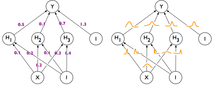
Probabilistic Programming (PP)
▪ allows automatic Bayesian inference
▪ on complex, user-defined probabilistic models
▪ utilizing “Markov chain Monte Carlo” (MCMC) sampling
▪ PyMC3
▪ a PP framework
▪ compiles probabilistic programs on-the-fly to C
▪ allows model specification in Python code
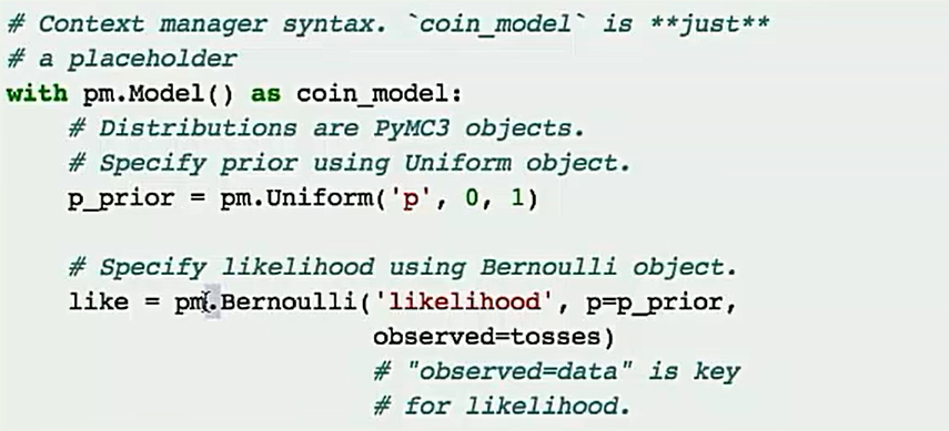
PyMC3:
statistical distributions
sampling algorithms
syntax
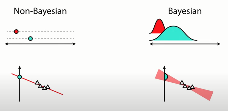


n번 동전을 던져서 h번 앞이 나온경우?
weak prior, strong prior를 가지는 경우를 생각한다.


------------------------------------------------------------------------------------------------------------
Estimating probabilities with Bayesian modelling in python

--------------------------------------------------------------------------------------------------------------
# observed data
np.random.seed(123)
n = 11
_a = 6
_b = 2
x = np.linspace(0, 1, n)
y = _a*x + _b + np.random.randn(n)
niter = 10000
with pm.Model() as linreg:
a = pm.Normal('a', mu=0, sd=100)
b = pm.Normal('b', mu=0, sd=100)
sigma = pm.HalfNormal('sigma', sd=1)
y_est = a*x + b
likelihood = pm.Normal('y', mu=y_est, sd=sigma, observed=y)
trace = pm.sample(niter, random_seed=123)
t = trace[niter//2:]
pm.traceplot(trace, varnames=['a', 'b'])
pass
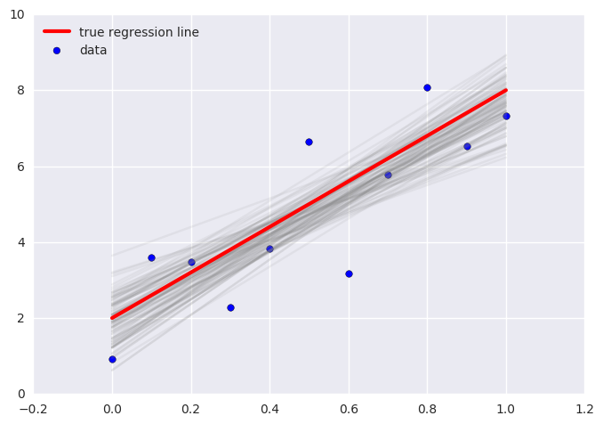
plt.scatter(x, y, s=30, label='data')
for a_, b_ in zip(t['a'][-100:], t['b'][-100:]):
plt.plot(x, a_*x + b_, c='gray', alpha=0.1)
plt.plot(x, _a*x + _b, label='true regression line', lw=3., c='red')
plt.legend(loc='best')
pass
--------------------------------------------------------------------------------------------------------------
%matplotlib inline
import pymc3 as pm
import numpy as np
import pandas as pd
import matplotlib.pyplot as plt
%config InlineBackend.figure_formats = ['retina']
plt.rc('font', size=12)
plt.style.use('seaborn-darkgrid')
# 1. load the stock returns data.
series = pd.read_csv('stock_returns.csv')
returns = series.values[:1000]
# 2. first, let's see if it makes sense to fit a Gaussian distribution to this.
with pm.Model() as model1:
stdev = pm.HalfNormal('stdev', sd=.1)
mu = pm.Normal('mu', mu=0.0, sd=1.)
pm.Normal('returns', mu=mu, sd=stdev, observed=returns)
with model1:
trace = pm.sample(500, tune=1000)
preds = pm.sample_posterior_predictive(trace, samples=500, model=model1)
y = np.reshape(np.mean(preds['returns'], axis=0), [-1])
--------------------------------------------------------------------------------------------------------------Bayesian_Linear_Regression.zip
--------------------------------------------------------------------------------------------------------------
Monte Carlo dropout
--------------------------------------------------------------------------------------------------------------